Log decrement (δ)
When a system is caused to oscillate and is then released from any external forcing functions (i.e., the system is then in free vibration), the amplitude decays because of loss within the system. The decay is exponential as given by the equation —
\begin{align} \label{eq:13401a} u = U e^{-(\delta \, f \, t)} \sin(2\pi \, f \, t) \end{align}
where —
| \( u \) | = instantaneous amplitude |
| \( U \) | = some peak amplitude |
| \( \delta \) | = log decrement |
| \( f \) | = frequency |
| \( t \) | = time |
(The exponent in equation \eqref{eq:13401a} is actually approximate but is nearly exact when \( \delta ≤ 2 \), which is appropriate for all ultrasonic systems.)
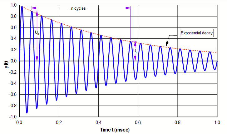
An example of equation \eqref{eq:13401a} is shown as the dotted line in figure 1. Note that larger values of \( \delta \) will cause the amplitude to decay more rapidly.
From equation \eqref{eq:13401a} it can be shown that if an amplitude maximum is measured at time \( t_0 \) and again later at time \( t_n \), the log decrement is given by (see figure 1) —
\begin{align} \label{eq:13402a} \delta = (1/n) \ln \left[ \frac{U_0}{U_n} \right] \end{align}
where —
| \( U_0 \) | = amplitude at time \( t_0 \) |
| \( U_n \) | = amplitude after \( n \) subsequent cycles |
| \( n \) | = number of cycles between \( U_0 \) and \( U_n \) |
|
|
|
Notes:
- The amplitudes \( U_0 \) and \( U_n \) can be any consistent type (peak or peak‑to‑peak). The above graph uses peak amplitudes for convenience.
- Any oscillation peak can be chosen to measure \( U_0 \).
- \( n \) is arbitrary. However, a large \( n \) will increase the calculation accuracy.
- As the difference between \( U_0 \) and \( U_n \) becomes smaller (i.e., a more slowly decaying amplitude), \( \delta \) also becomes smaller.
For the example of figure 1 the log decrement is —
\begin{align} \label{eq:13403a} \delta &= (1/10) \ln \left[ \frac{0.889}{0.346} \right] \\[0.7em]%eqn_interline_spacing &= 0.094 \nonumber \end{align}
Note: Figure 1 shows a starting amplitude of 0 at \( t = 0 \) but this is arbitrary. The calculated \( \delta \) does not depend on the starting amplitude. This can be seen by imagining the entire amplitude waveform being shifted left or right.
Relation to Q
\( \delta \) and Q (quality factor) are related by —
\begin{align} \label{eq:13404a} Q = \frac{\pi}{\delta} \end{align}
Thus, when \( \delta \) is small (a slowly decaying amplitude) \( Q \) is large.
Also see —
Attenuation
Bandwidth
Damping ratio
Loss tangent