Pochhammer Amplitude Distributions
in an Infinitely Long Cylinder

---

In 1876, Pochhammer originally developed the equations for wave propogation in an infinitely long elastic cylinder with isotropic material properties. These equations predict the axial and radial amplitude distributions. (Note: the Pochhammer solution is sometimes called the Pochhammer-Chree solution or the Pochhammer-Love solution.)

The following has been taken essentially from Zemanek[1A]).

Axial amplitude distribution

For a cylinder of radius R, the axial amplitude \( U_{axial} \) at a radial distance \( r \) from the center of the cylinder is given by the following equation. (See Zemanek[1A], p. 271, lower equation 18.)

\begin{align} \label{eq:11001a} {U_{axial}}(r) = \Big[2 \, (\gamma \, R)^2 - \Omega^2 \Big] J_1(k \, R) \, J_0(h \, r) + \Big[ 2 \, (k \, R) \, (h \, R) \, J_1(h \, R) \, J_0(k \, r) \Big] \end{align}

where —

\begin{align} \label{eq:11001a1} \tag{1a} \gamma = \frac{2 \pi \, f}{c} \end{align}

\begin{align} \label{eq:11001a2} \tag{1b} \Omega = \frac{2 \pi \, f \, R}{c_s} \end{align}

\begin{align} \label{eq:11001a3} \tag{1c} h = 2 \pi \, f \, \left[ \frac{1}{{c_d}^2} - \frac{1}{{c}^2} \right]^{1/2} \end{align}

\begin{align} \label{eq:11001a4} \tag{1d} k = 2 \pi \, f \, \left[ \frac{1}{{c_s}^2} - \frac{1}{{c}^2} \right]^{1/2} \end{align}

\begin{align} \label{eq:11001a5} \tag{1e} c_s = c_{tw} \left[ \frac{1}{2 \, (1 + \nu)} \right]^{1/2} \end{align}

\begin{align} \label{eq:11001a6} \tag{1f} c_d = c_{tw} \left[ \frac{1 - \nu}{(1 + \nu) \, (1 - 2\nu)} \right]^{1/2} \end{align}

\begin{align} \label{eq:eq:11001a7} \tag{1g} c_{tw} = \left[ \frac{E}{\rho} \right]^{1/2} \end{align}

where —

\( U_{axial}(r) \)	= axial amplitude at radius \( r \)
\( r \)	= radius at which the amplitude will be evaluated
\( R \)	= radius of cylinder
\( f \)	= frequency
\( c \)	= effective wave speed of the cylinder whose radius is \( R \)
\( c_{tw} \)	= thin-wire wave speed
\( c_s \)	= shear wave speed
\( c_d \)	= dilitational wave speed
\( \nu \)	= Poisson's ratio
\( J_0 \)	= Bessel function of the first kind, order 0
\( J_1 \)	= Bessel function of the first kind, order 1

Each Bessel function operates on the parameter in ( ) (i.e., the Bessel function argument). (See Appendix A for further notes on Bessel functions.)

\( c_s \) and \( c_d \) can be evaluated from various material constants. (See the chapter on "Wave Motion".) However, unlike \( c_s \) and \( c_d \), \( c \) is not a material constant. Instead, \( c \) depends on the cylinder diameter. For the chosen cylinder diameter, \( c \) can be determined from the Pochhammer frequency equation. (See Zemanek[1A], p. 267, equation 6. Also see the chapter on "Wave Motion".) However, the solution of this equation is difficult. Instead, \( c \) can more easily be determined by the Mori equation. (See the chapter on "Wave Motion".)

Note that both \( c_s \) and \( c_d \) depend on Poisson's ratio \( \nu \). Hence, the axial amplitude distribution as well as the radial amplitude (below) will also depend on Poisson's ratio.

In the above equation, if \( r = 0 \) then \( U \) represents the axial amplitude at the axis of the cylinder. For \( r = 0 \) two of the Bessel functions evaluate to 1:

\begin{align} \label{eq:11002a} J_0(h \, r) = J_0(0) = 1 \end{align}

\begin{align} \label{eq:11003a} J_0(k \, r) = J_0(0) = 1 \end{align}

Then, the axial amplitude at the center of the cylinder is —

\begin{align} \label{eq:11004a} {U_{axial}}(r=0) = \Big[2 \, (\gamma \, R)^2 - \Omega^2 \Big] J_1(k \, R) + \Big[ 2 \, (k \, R) \, (h \, R) \, J_1(h \, R) \Big] \end{align}

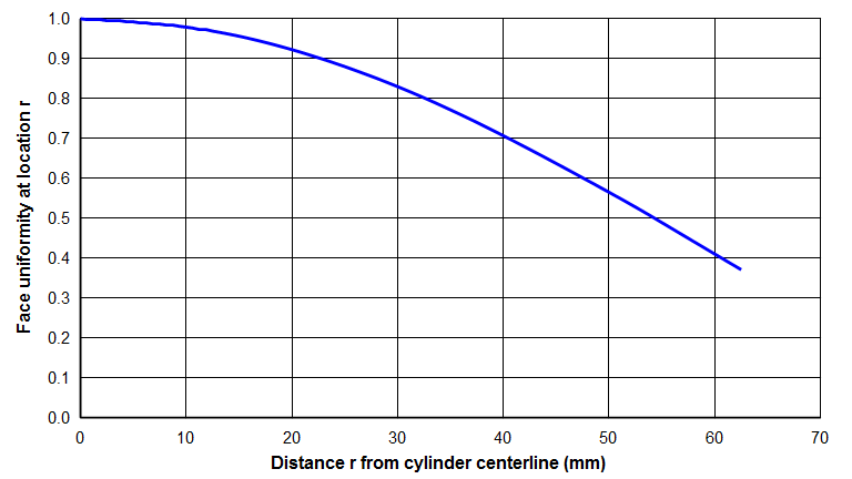
If equation \eqref{eq:11001a} is evaluated at \( r \) and divided by equation \eqref{eq:11004a}, the result is \( \widehat{U}(r) \) (i.e., the uniformity at radius \( r \)):

\begin{align} \label{eq:11005a} \widehat{U}(r) = \frac{\textsf{Equation \eqref{eq:11001a} @ r}}{\textsf{Equation \eqref{eq:11004a}}} \end{align}

Equation \eqref{eq:11005a} is graphed in figure 1 for a Ø125 mm Al 7075‑T6 cylinder that vibrates axially at 20 kHz.

Figure 1. Pochhammer uniformity across a 20 kHz Ø125 mm Al 7075‑T6 cylinder

Evaluating equation \eqref{eq:11005a} at \( R \) (the cylinder periphery) gives the overall uniformity \( \widehat{U} \).

\begin{align} \label{eq:11006a} \widehat{U} = \frac{\textsf{Equation \eqref{eq:11001a} @ R}}{\textsf{Equation \eqref{eq:11004a}}} \end{align}

If equation \eqref{eq:11006a} is evaluated for cylinders of various diameters, a typical result is shown in figure 2.

Figure 2. Pochhammer face uniformity for an Al 7075‑T6 cylinder

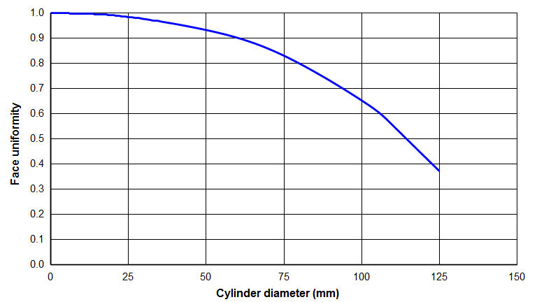
Note: see Appendix B for a simpler cubic equation that approximates equation \eqref{eq:11006a}.

Radial amplitude distribution

For a cylinder of radius \( R \), the radial amplitude \( U_{radial} \) at a radial distance \( r \) from the center of the cylinder is given by the following equation. (See Zemanek[1A], p. 271, upper equation 18.)

\begin{align} \label{eq:11007a} {U_{radial}}(r) = \Big[ \frac{h}{\gamma} \Big] \bigg\{ \Big[ 2 \, (\gamma \, R)^2 - \Omega^2 \Big] J_1(k \, R) \, J_1(h \, r) - \Big[ 2 \, (\gamma \, R)^2 \, J_1(h \, R) \, J_1(k \, r) \Big] \bigg\} \end{align}

At the periphery of the cylinder \( r = R \) the above equation becomes —

\begin{align} \label{eq:11008a} {U_{radial}}(r=R) = \Big[ \frac{h}{\gamma} \Big] \bigg\{ \Big[ 2 \, (\gamma \, R)^2 - \Omega^2 \Big] J_1(k \, R) \, J_1(h \, R) - \Big[ 2 \, (\gamma \, R)^2 \, J_1(h \, R) \, J_1(k \, R) \Big] \bigg\} \end{align}

If equation \eqref{eq:11008a} is divided by equation \eqref{eq:11004a} then the result is the relative radial amplitude (as a percent of the axial centerline amplitude):

\begin{align} \label{eq:11009a} \widehat{U}_{radial} = \frac{\textsf{Equation \eqref{eq:11008a} @ R}}{\textsf{Equation \eqref{eq:11004a}}} \end{align}

It turns out that the numerator and denominator of this equation have opposite signs. This indicates that when the face is moving outward the node is collapsing inward and vice versa. This is expected from Poisson coupling.

(Note: See Mori (1) for other equations that approximate the face amplitude distribution in a cylindrical horn.)

Maximum applicable diameter for half-wave horns

The Pochhammer equation was developed for an infinitely long cylinder. However, cylindircal horns have finite length. It turns out that the Pochhammer equation is valid for cylindrical horns as long as the shear stresses are small compared to the longitudinal stresses. This will be true if the horn diameter is not excessively large compared to the tuned half-wavelength. Zemanek[1A] (pp. 272 - 275) shows that the shear stresses remain less than 1% of the longitudinal stress as long as \( \Omega \) < 2.6 (p. 275)). (Also see Thurston, p. 16.) Substituting this value and \( c_s \) (equation \eqref{eq:11001a5}) into equation \eqref{eq:11001a2} and solving for \( D \) (i.e., \( 2R \)) gives:

\begin{align} \label{eq:11010a} D &\leq \Gamma_{tw} \, \left[ \frac{5.2}{\pi} \right] \, \left[ \frac{1}{2 \, (1 + \nu)} \right]^{1/2} \\[0.7em]%eqn_interline_spacing &\leq \left[ \frac{c_{tw}}{2 \, f} \right] \, \left[ \frac{5.2}{\pi} \right] \, \left[ \frac{1}{2 \, (1 + \nu)} \right]^{1/2} \nonumber \end{align}

where —

\( D \)	= diameter of cylinder
\( f \)	= frequency
\( c_{tw} \)	= thin-wire wave speed
\( \Gamma_{tw} \)	= material thin-wire half-wavelength
\( \nu \)	= Poisson's ratio

Using the material constants for Al 7075‑T6 aluminum ( \( c_{tw} \) = 5081 m/sec, \( \nu \) = 0.33), the above equation indicates that the maximum diameter for which the Pochhammer equation is valid for this aluminum at 20 kHz is approximately 130 mm. Above 130 mm, the Pochhammer equation will have increased error. In fact, the Pochhammer equation predicts that the aluminum horn will a node at 150 mm. This is obviously incorrect, since an axial resonance should never have a face node (except when influenced by an adjacent nonaxial resonance).

In addition to the limiting diameter, the Pochhammer equation also assumes that the rod material is homogeneous. Therefore, it does consider the effect of a stud.

---

Appendix A — Bessel Functions

The important Bessel functions for the Pochhammer equation have the following characteristics (see Kinsler, appendix A4, pp. 449 - 452) —

1. J₀(x), where \( x \) is a real number — The \( J_0(x)\) function resembles a decaying cosine function and has a maximum value of 1.0.
2. \( J_0(jx) \), where \( jx \) is an imaginary number — The \( J_0(jx)\) function is real valued and resembles a hyperbolic cosine function, whose value rapidly increases as \( x \) increases. \( J_0(jx)\) can be expressed as a modified Bessel function \( I_0(x)\) (Kinsler, p. 450) —
   
   

   \begin{align} \label{eq:11035a} J_0(jx) = I_0(x) \end{align}

   where \( I_0(x)\) is real valued.
3. J₁(x), where \( x \) is a real number — The \( J_1(x)\) function resembles a decaying sine function and has a maximum value of about 0.58.
4. \( J_1(jx) \), where \( jx \) is an imaginary number — The \( J_1(jx) \) function is imaginary and resembles a hyperbolic cosine function, whose value rapidly increases as \( x \) increases. \( J_1(jx) \) can be expressed as a modified Bessel function (Kinsler, p. 450) —
   
   

   \begin{align} \label{eq:11036a} J_1(jx) = j I_1(x) \end{align}

   where \( I_1(x)\) is real valued.

For longitudinal resonators that are of interest in high-power ultrasonics, \( c_d \) is always greater than \( c \). Thus, \( h \) from equation \eqref{eq:11001a3} is imaginary since the value under the \( \sqrt{\textsf{ }} \) in equation \eqref{eq:11001a3} is negative. Thus, \( (h \, R) \) and \( J_1(h \, R) \) are both imaginary and their product in the above equations is thus a negative real number.

---

Appendix B — Polynomial Curve-fit

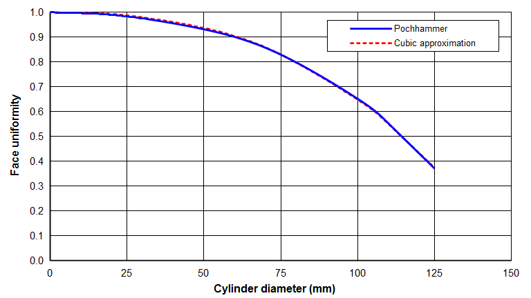
While equation \eqref{eq:11006a} agrees well with measured uniformities, it can be cumbersome to calculate. Therefore, a cubic polynomial equation has been fitted —

\begin{align} \label{eq:11031a} \widehat{U} = 1 + b_2 \, \left( \frac{D}{\Gamma_{tw}} \right)^2 + b_3 \, \left( \frac{D}{\Gamma_{tw}} \right)^3 \end{align}

where —

\( \widehat{U} \)	= cylinder uniformity for specified cylinder diameter
\( D \)	= cylinder diameter
\( \Gamma_{tw} \)	= thin-wire half-wavelength
\( b_2 \), \( b_3 \)	= curve fit constants

Note that as the cylinder diameter goes to zero the uniformity goes to 1.0, as required. Also, since the slope of the uniformity curve should be zero when the horn diameter is zero, the equation has no linear term \( \left( D / \Gamma_{tw} \right)^1 \) (or, alternately, the coefficient \( b_1 \) of the linear term is 0).

The thin-wire half-wavelength \( \Gamma_{tw} \) is calculated from the equation —

\begin{align} \label{eq:11032a} \Gamma_{tw} = \frac{c_{tw}}{2 \, f} \end{align}

Equation \eqref{eq:11031a} was fitted to the Pochhammer equation for 7 diameters ranging between 0 and 125 mm at a frequency of 20 kHz with a wave speed of 5081 and Poisson's ratio of 0.33 (corresponding to Al 7075‑T6 aluminum). This yielded the curve-fit constants —

\begin{align} \label{eq:11033a} b_2 = -0.24744 \end{align}

\begin{align} \label{eq:11034a} b_3 = -0.40538 \end{align}

with a the standard error of estimate 0.32.

Equation \eqref{eq:11031a} with the fit constants from \eqref{eq:11033a} and \eqref{eq:11034a} is graphed in figure B1.

Figure B1. Pochhammer face uniformity for a 20 kHz Al 7075‑T6 cylinder

If the material properties vary significantly from the above assumed values then the calculated uniformity will err. Fortunately, most acoustic materials have material properties that are reasonably close to aluminum so equation \eqref{eq:11031a} should give reasonable results for these materials.